はじめに
前回は、MVTec-Anomaly-Detection をカスタムデータで学習させる方法について説明しました。
今回は、カスタムデータで学習させたモデルの検出結果をしきい値を変化させて、確認していきます。
前提条件
前提条件は以下の通りです。
- Tensoflow == 2.9.3
- numpy == 1.23.5
- ktrain == 0.33.2
- Windows11
- Python3.10
test.py の変更
検出に使用した test.py を変更していきます。
test.py の 120 行目付近を変更します。
threshold_ = validation_result["best_threshold"]
threshold = 0.5
print("\nthreshold {:4} to {}\n".format(threshold_, threshold))
しきい値を 0.5 に設定しました。
以下のコマンドで実行します。
python test.py -p .\saved_models\data\custom\mvtecCAE\ssim\17-02-2023_06-59-39\mvtecCAE_b12_e99.hdf5 -sすると、スコアは 0.53 と 0.1 上昇しましたが、不良の感度が高くなり、良品画像の誤検知が少し増えています。
さらに精度を上げるには
さらに精度を上げるには、学習する画像 ( good ) を、選別する必要があります。
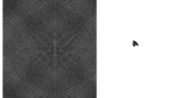
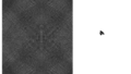
今回使用した工業製品画像の Class1 を見てもらうと、背景の模様が一様でなく、様々なパターンがあることが分かります。
今回は強引なやり方ですが、これを選別します。
Class1 の 891.png と、Class1_def の 19.png を残して他は削除してください。
891.png を適当に 10 枚ほどコピーしてください。これを good とします。
test の画像も適当に 5 枚ほどコピーしてください。
極端に good の画像が少ないと、エラーが発生します。
これで学習を実行します。
python train.py -d data/custom -a mvtecCAE -b 2 -l mssim -c rgbファインチューニングします。
python finetune.py -p .\saved_models\data\custom\mvtecCAE\mssim\18-02-2023_21-37-47\mvtecCAE_b2_e99.hdf5 -m ssim -t float64test.py を実行します。threshold は元に戻しておいてください。
python test.py -p .\saved_models\data\custom\mvtecCAE\mssim\18-02-2023_21-37-47\mvtecCAE_b2_e99.hdf5 -s filenames predictions truth accurate_predictions
0 defect\19 (1).png 0 1 False
1 defect\19 (2).png 0 1 False
2 defect\19 (3).png 0 1 False
3 defect\19 (4).png 0 1 False
4 defect\19 (5).png 0 1 False
5 defect\19 (6).png 0 1 False
6 good\891 (1).png 0 0 True
7 good\891 (2).png 0 0 True
8 good\891 (3).png 0 0 True
9 good\891 (4).png 0 0 True
10 good\891 (5).png 0 0 True
11 good\891 (6).png 0 0 True全然検出できていません。ここで、先ほどの方法で test.py を変更します。
threshold_ = validation_result["best_threshold"]
threshold = 0.6
print("\nthreshold {:4} to {}\n".format(threshold_, threshold))
上記に変更して再度検出を実行すると、good が True, defect が False として検出されました。
            filenames  predictions  truth  accurate_predictions
0   defect\19 (1).png            0      1                 False
1   defect\19 (2).png            0      1                 False
2   defect\19 (3).png            0      1                 False
3   defect\19 (4).png            0      1                 False
4   defect\19 (5).png            0      1                 False
5   defect\19 (6).png            0      1                 False
6    good\891 (1).png            1      0                 False
7    good\891 (2).png            1      0                 False
8    good\891 (3).png            1      0                 False
9    good\891 (4).png            1      0                 False
10   good\891 (5).png            1      0                 False
11   good\891 (6).png            1      0                 False
あとはこの結果を反転させるだけで、良品 / 不良品の判別ができるようになります。
異常検出の面積で判定したいとき
しきい値のみで分別が難しい場合、異常部分の面積で不良を判別することができます。
test.py の、32 行目を以下のように変更してください。
def is_defective(areas, min_area):
    """Decides if image is defective given the areas of its connected components"""
    areas = np.array(areas)
    if areas[areas >= min_area].shape[0] > 16:   ←ここを 0 から 16 に変更
        return 1
    return 0
areas[areas >= min_area].shape[0] で、異常部分の面積 (px) を算出しています。
今回は面積 16 以上を不良として判別します。
また、test.py の 120 行目付近は以下のようにしてください。
threshold_ = validation_result["best_threshold"]
threshold = 0.9
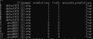
print("\nthreshold {:4} to {}\n".format(threshold_, threshold))上記のように変更し、test.py を実行すると、以下の出力が得られます。
            filenames  predictions  truth  accurate_predictions
0   defect\19 (1).png            1      1                  True
1   defect\19 (2).png            1      1                  True
2   defect\19 (3).png            1      1                  True
3   defect\19 (4).png            1      1                  True
4   defect\19 (5).png            1      1                  True
5   defect\19 (6).png            1      1                  True
6    good\891 (1).png            0      0                  True
7    good\891 (2).png            0      0                  True
8    good\891 (3).png            0      0                  True
9    good\891 (4).png            0      0                  True
10   good\891 (5).png            0      0                  True
11   good\891 (6).png            0      0                  True
綺麗に判別できています!
おわりに
今回は、しきい値の変更と面積の変更で検出精度をより良くする方法について説明しました。
Tensorflow で書かれているので完全に中身を理解できませんでしたが、次は PyTorch の実装を紹介できたらと思います。

コメント